그림을 그립시다 The Joy of ggplotting: compositional bar plots

First of all, download a publicly available dataset from kaggle https://www.kaggle.com/bbhatt001/human-microbiome-project

library(tidyverse)  
d0 <- read_csv("project_catalog.csv")
dim(d0)

## [1] 2915   17

names(d0)

##  [1] "HMP ID"                  "GOLD ID"                
##  [3] "Organism Name"           "Domain"                 
##  [5] "NCBI Superkingdom"       "HMP Isolation Body Site"
##  [7] "Project Status"          "Current Finishing Level"
##  [9] "NCBI Submission Status"  "NCBI Project ID"        
## [11] "Genbank ID"              "Gene Count"             
## [13] "IMG/HMP ID"              "HOMD ID"                
## [15] "Sequencing Center"       "Funding Source"         
## [17] "Strain Repository ID"

table(d0$`HMP Isolation Body Site`) 

## 
##                airways                  blood                   bone 
##                    236                     75                     27 
##                    ear                    eye gastrointestinal_tract 
##                      4                      8                    745 
##                  heart                  liver            lymph_nodes 
##                      2                      1                      1 
##                   nose                   oral                  other 
##                      2                    347                     13 
##                   skin                unknown       urogenital_tract 
##                    267                    654                    529 
##                  wound 
##                      4

We subset the data to include only body sites with sufficient data:

d <- d0 %>%
  filter(`HMP Isolation Body Site` %in% c("airways", "gastrointestinal_tract",
                                          "oral", "skin", "urogenital_tract")) %>%
  mutate(`Body site` = factor(`HMP Isolation Body Site`)) %>%
  mutate(Genus = str_extract(`Organism Name`, "^[^\\s]+")) %>% # extract the string before the first space
  count(`Body site`, Genus) %>%
  pivot_wider(Genus, names_from = `Body site`, values_from = "n", values_fill = list(n = 0)) 

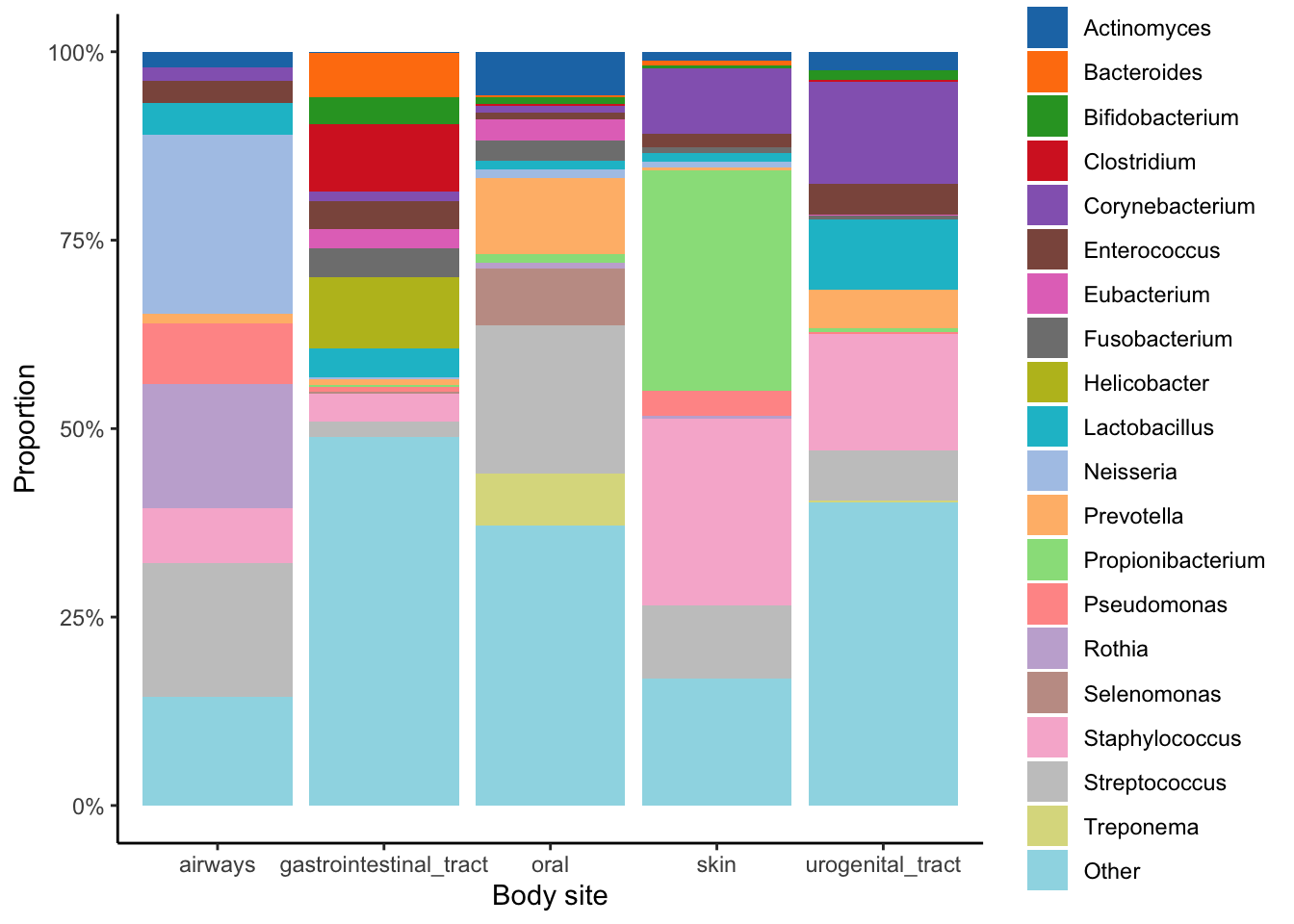
Proportion of genera in each body site:

num_top <- 19 # plus "Other" will make 20
prop <- d %>%
  column_to_rownames("Genus") %>%
  sweep(2, colSums(.), "/")

meanProp <- apply(prop, 1, mean) %>% sort(decreasing = T) 
topGenus <- names(meanProp[1:num_top])
print(topGenus)

##  [1] "Streptococcus"     "Staphylococcus"    "Propionibacterium"
##  [4] "Corynebacterium"   "Neisseria"         "Lactobacillus"    
##  [7] "Rothia"            "Prevotella"        "Enterococcus"     
## [10] "Pseudomonas"       "Actinomyces"       "Helicobacter"     
## [13] "Clostridium"       "Fusobacterium"     "Selenomonas"      
## [16] "Treponema"         "Bacteroides"       "Bifidobacterium"  
## [19] "Eubacterium"

d2 <- d %>%
  mutate(Genus = ifelse(Genus %in% topGenus, Genus, "Other")) 

propNew <- rowsum(d2 %>% select(-Genus), d2$Genus) %>%
  sweep(2, colSums(.), "/") %>%
  rownames_to_column("Genus") %>%
  pivot_longer(-Genus, names_to = "Body site", values_to = "Proportion") %>%
  mutate(Genus = fct_relevel(Genus, "Other", after = Inf)) 

Now fun part:

library(ggsci)
g <- propNew %>%
  ggplot(aes(x = `Body site`, y = Proportion)) +
  geom_col(aes(fill = Genus)) +
  scale_fill_d3(palette = "category20") +
  scale_y_continuous(labels = scales::percent) +
  theme_classic() 

print(g)